



 Key Findings
A sales forecast is only as reliable as the system feeding it. The most accurate forecasts are not built from complex formulas. They are the natural outcome of a clean ICP, verified contact data, signal-based outreach, and consistent follow-up. Fix the inputs and the forecast fixes itself.
Intent-based forecasting is the most powerful model for outbound teams because it focuses on what prospects are doing right now, not what happened last quarter. A company that just raised funding, is hiring a sales team, and switched CRMs is not just a good fit. It is an active buyer with a window that closes fast.
Pipeline velocity is the diagnostic tool most teams are missing. It does not just tell you if you are on track. It tells you exactly which stage deals are stalling in, so you can fix the specific problem instead of blaming the whole process.
Multi-touch attribution changes how you allocate resources. Giving 100% credit to the last touchpoint is the fastest way to cut channels that are silently driving conversions. Email, LinkedIn, and cold calling work together. Our data shows 68% of conversions at Reachly involve all three channels.
Most forecasting problems are actually pipeline generation problems in disguise. If you cannot predict your reply rate, your meeting book rate, or your close rate for a specific segment, the issue is not your spreadsheet. It is the outbound system that is supposed to be producing those numbers consistently.
A sales forecasting example is a worked projection that turns a known conversion chain into a revenue number, and the nine models on this page each carry one. On one live Reachly engagement the chain was 85 qualified leads over six months, a 7.1% close rate, and 6 closed deals, which forecasts almost exactly one new deal per month at steady state. That is the whole job: measure what your pipeline already does, then multiply it forward.
Most B2B forecasts miss because they start from a quota and work backwards. The nine models below start from pipeline behavior you can already observe, deal speed, buying signals, reply rates, and territory coverage, and each one carries a worked calculation you can copy into a spreadsheet this afternoon.
Forecasting reads the pipeline you already have. To plan the pipeline you still need, Reachly's pipeline generation guide has a worksheet that turns a quarterly target into meetings per month.
We run these models across outbound campaigns for B2B teams, so the numbers here come from campaigns we operate rather than from a textbook. Where a figure is illustrative, it says so.
TL;DR: Summary
- A sales forecast is a conversion chain multiplied forward. Leads, meeting rate, close rate, average deal value, and cycle length are the only five inputs most B2B teams need.
- Pipeline velocity is the fastest diagnostic. Opportunities times deal value times win rate, divided by cycle length in days, gives a daily revenue run rate you can project across a quarter.
- Intent-based forecasting is the most accurate model for outbound, because a funding round or a hiring spike tells you an account is in market now rather than that it converted last year.
- Weighted pipeline forecasting by opportunity stage is the fastest model to stand up, because it reuses CRM stages you already have. Derive the stage probabilities from your own closed-won history, never from a CRM default.
- Time series and moving average forecasting is the model to use once outbound reaches steady state, which is around month 5. Three months of history is the floor and twelve is where seasonality becomes visible.
- Forecast accuracy is measured as 1 minus the absolute error over actual revenue. Anything above 85% is a working forecast, and below 70% the inputs are the problem, not the formula.
- Outbound pipeline does not become forecastable on day one. Campaigns launch around week 4, first meetings come by week 5 to 6, or within 10 days on pre-warmed domains, and volume is predictable from month 3.
- Across one six-month engagement the funnel produced 85 qualified leads, 6 closed deals, and a 4.57x return, which is enough history to forecast the next quarter within a deal.
- If a forecast keeps breaking, the fix is upstream in list quality, signal timing, and follow-up consistency. We build that system as part of our B2B appointment setting services.
What does a complete sales forecasting example look like?
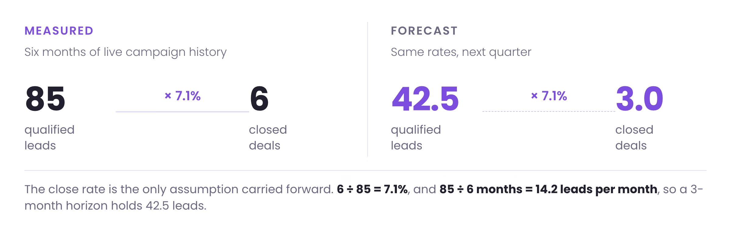
A forecast is a conversion chain with a number attached to every step. Below is the chain from an engagement we can show publicly, our work with Primal, a marketing services firm in Thailand. Six months of outbound produced 85 qualified leads and 6 closed deals at a 4.57x return, with customer acquisition cost down 35%.
Those two published numbers are enough to forecast the next quarter. 6 deals divided by 85 qualified leads is a 7.1% close rate. 85 leads over six months is 14.2 qualified leads per month. Multiply the two and steady state is 1.0 closed deal per month, so a full quarter at the same inputs forecasts 42.5 qualified leads and 3 closed deals.
| Step | Observed over 6 months | Monthly rate | Next quarter forecast |
|---|---|---|---|
| Qualified leads | 85 | 14.2 | 42.5 |
| Close rate | 6 of 85 | 7.1% | 7.1% |
| Closed deals | 6 | 1.0 | 3.0 |
| Return on spend | 4.57x | 4.57x | 4.57x |
| Time to break even | 3 months | n/a | already past |
Source: the published Primal case study. Two caveats before you copy the method. A single quarter of history is thin, so widen the range rather than quoting one figure, and the first three months of any outbound program sit below steady state while infrastructure warms up.
The three formulas behind every forecast on this page
Every model further down reduces to one of three calculations. Each is worked here with real arithmetic so you can check your own numbers against the method.
1. Pipeline velocity. Multiply open opportunities by average deal value and win rate, then divide by the sales cycle in days. With 40 open opportunities, an $18,000 average deal, a 22% win rate, and a 75-day cycle: 40 times 18,000 is 720,000, times 0.22 is 158,400, divided by 75 is $2,112 of pipeline per day. Across a 90-day quarter that forecasts $190,080.
2. Weighted pipeline. Multiply each open deal by the historical close rate of the stage it sits in, then add the results. Ten deals worth $20,000 each at a 30% stage close rate contribute $60,000, not $200,000. Use close rates you measured, not the default percentages your CRM shipped with.
3. Forecast accuracy. Subtract the forecast from actual revenue, take the absolute value, divide by actual revenue, and subtract the result from 1. Forecast $250,000 against $220,000 actual and the error is $30,000, which is 13.6% of actual, so accuracy is 86.4%. Track this every quarter. It is the only number that tells you whether the rest of the exercise is working.
Illustrative figures in this section are marked as such. The Primal numbers are published on the case study page.
1. Pipeline Velocity Forecasting
If your sales pipeline is a black box where deals go in and revenue might come out, pipeline velocity forecasting is your flashlight. It stops you from counting open opportunities and forces you to measure the speed at which deals move from one stage to the next. This is a critical example of sales forecasting because it focuses on momentum, not just volume. The core idea is simple: how fast are we turning a new lead into a closed deal?
This method calculates your sales velocity with four metrics: the number of opportunities, average deal size, your win rate, and the length of your sales cycle. Tracking these components gives you a real-time health check on your sales process. A drop in velocity tells you something is wrong before your revenue takes a hit.
Why It Works for B2B Outbound
Pipeline velocity is especially powerful for agencies like Reachly that manage multichannel outbound campaigns. We track how quickly a prospect moves from an initial email reply to a LinkedIn connection, a phone call, and finally, a qualified meeting. That timeline is a direct measure of campaign effectiveness, stage by stage.
If velocity slows between the "LinkedIn Touchpoint" and "Phone Call" stages, we know exactly where the bottleneck is. Maybe the LinkedIn messaging is not working, or the SDRs need better context for their calls. This granular view lets us fix problems in a specific stage without guessing.
Pipeline velocity turns your sales process into a diagnostic tool. Instead of seeing a low final number, you see where the process broke down and why.
Actionable Tips for Implementation
- Define your stages clearly: Your pipeline stages must reflect the actual steps a buyer takes. If "Initial Contact" and "Discovery Call" are the same thing, your data is useless. Map stages to concrete actions like "Demo Scheduled" or "Proposal Sent."
- Track source-specific velocity: Not all leads are equal. A cold email lead moves at a different speed than one from a targeted LinkedIn sequence. Track velocity for each channel separately to see what actually works.
- Use moving averages: A single great week or a bad month can skew your forecast. Use a 30 or 60-day moving average for your win rates and deal cycle length to get a stable prediction. This helps you avoid knee-jerk reactions.
2. Intent-Based Demand Forecasting with Buying Signals
Relying on historical sales data is like driving while looking in the rearview mirror. Intent-based demand forecasting flips the script by focusing on what your ideal customers are doing right now. It shifts your attention from past performance to future behavior, making it a powerful example of sales forecasting for proactive teams. The goal is to find and engage accounts showing early signs they are ready to buy, often before they even start looking.
This method tracks real-time buying signals like recent funding rounds, spikes in hiring for specific roles, tech stack changes, or significant headcount growth. Instead of waiting for a lead to fill out a form, you find them the moment their needs change. This lets you forecast demand from a pool of high-intent accounts far more likely to convert.
Tracking those signals reliably takes a system behind it: sources mapped, records enriched, and changes pushed into the forecast the week they happen. That build work sits inside GTM engineering, the function that owns the data plumbing feeding a signal-based forecast.
Why It Works for B2B Outbound
Intent-based forecasting is the engine behind modern outbound agencies like Reachly. We do not just build a list of companies in an industry. We build a list of companies showing clear signals of expansion and need. For example, we find businesses that just raised a Series A and are now hiring their first sales team. That combination describes a company with a problem we can solve this quarter.
This approach gives our outreach immediate context. Instead of a generic pitch, our first message can reference their specific growth signal: "Saw you are hiring 10 new account executives after your funding round." This instantly separates our outreach from the noise. It shows we did our homework and makes the conversation about their goals, not our service.
Reachly's signal stack in practice: For Primal, we built five separate campaigns each triggered by a different signal: companies hiring for a marketing role, companies that had just raised funding, companies with dropping organic traffic, and companies not ranking on page one. Each signal told us something different about the prospect's pain level. Those campaigns hit 8% positive reply rates within the first month.
Buying signals turn cold outreach into warm, relevant conversations. You stop guessing who might need you and start talking to people who are actively trying to solve a problem you can fix.
Actionable Tips for Implementation
- Establish a signal scoring matrix: Not all signals are equal. Define what matters most. A recent funding round might be weighted at 30%, while 25% headcount growth gets 25%, and a specific tech stack change gets 20%. Score and prioritize accounts.
- Combine signals for higher confidence: One signal is interesting. Two or three signals from the same account is a call to action. An account that just got funding, is hiring salespeople, and adopted a new CRM is a high-priority target that needs immediate, personalized outreach.
- Time your outreach: Intent signals have a short shelf life. The best time to reach out is within two to four weeks of a signal. This is when budgets are being set and strategies are being formed. Wait too long, and your competitors get there first.
- Validate your signals: Continuously track which signals actually lead to closed deals. You might find that for your product, headcount growth is a far better predictor of a sale than a funding announcement. Use this data to refine your scoring model.
3. Cohort Analysis and Campaign Performance Forecasting
If you want the same arithmetic applied to spend rather than deals, our cold email ROI calculator walks through forecasting pipeline from a cold email budget.
If you launch outbound campaigns with your fingers crossed, cohort analysis is how you build predictability. Instead of treating every campaign like a new experiment, this method groups prospects by shared traits like industry, company size, or a specific buying signal. This is a powerful example of sales forecasting because it uses past performance to predict future results with high accuracy.
You are no longer guessing. You are benchmarking.
The method tracks how these defined groups move through your outreach funnel. By analyzing past campaigns targeting, for example, Series B SaaS companies, you can forecast the reply rates, meetings booked, and deal flow for a new campaign targeting the same segment. It replaces wishful thinking with data.
Why It Works for B2B Outbound
Cohort analysis is essential for an agency like Reachly, where we run dozens of unique multichannel campaigns. It lets us give clients a realistic forecast based on real data, not just industry averages. For instance, we can confidently predict that a LinkedIn-first sequence targeting companies with recent funding signals will yield a 3-5% reply rate because we have run that exact play before and tracked the results.
This approach also helps us diagnose campaign performance. If a new campaign for MarTech companies is underperforming against its historical cohort benchmark, the audience is already validated, so the likely fault is the new messaging or sequence structure, letting us fix the variable that changed instead of blaming the entire strategy.
Cohort analysis isolates variables. It turns your campaign history into a reliable benchmark, letting you test new messaging while forecasting outcomes based on what you already know works.
Actionable Tips for Implementation
- Document every campaign parameter: Be militant about tracking your targeting criteria. Document the industry, company size, buying signals, messaging angles, and sequence length for every cohort you build.
- Track key metrics per cohort: For each group, measure open rates, click rates, reply rates, qualified replies, and meetings booked. This creates the benchmarks you will use for forecasting.
- Create and revisit benchmarks: Group your historical data by campaign type and review these benchmarks quarterly. Your market changes, and so will your results.
4. Territory and Account-Based Forecasting (ABM Approach)
If your total addressable market feels like an ocean, territory forecasting is how you start drawing maps. Instead of looking at your entire pipeline, this method forces you to predict outcomes for specific segments: geographic regions, industries, or defined account lists. It stops you from applying a single win rate across different customer profiles. This is a powerful example of sales forecasting because it ties your predictions directly to your market penetration strategy.
This approach breaks down your forecast into manageable chunks. You predict revenue for the Midwest Fortune 500 territory, or the "Healthcare SaaS" vertical. The forecast becomes a reflection of how well you can activate a specific market segment.
Why It Works for B2B Outbound
Territory forecasting is essential for outbound agencies like Reachly because our success depends on precision targeting. We do not blast emails into the void. We build hyper-specific campaigns for defined market segments. For example, we might forecast that a well-mapped healthcare vertical with 500 qualified accounts will yield 15-20 qualified leads over eight weeks. That prediction rests on verified contact data quality and historical engagement rates for that industry.
This method allows us to set clear expectations and measure performance accurately. If our campaign targeting Midwest manufacturing companies is underperforming against the forecast, we know the issue lies with the messaging, offer, or contact data for that segment. We do not have to overhaul our entire outbound strategy. We can diagnose the problem with surgical precision.
Territory forecasting links your sales predictions directly to your market strategy. A bad forecast doubles as a signal that your read on a specific market segment is flawed.
Actionable Tips for Implementation
- Invest in accurate TAM mapping: Use a multi-source approach, like Reachly's 10+ data source methodology, to build a clean, verified list of target accounts within each territory. Garbage in, garbage out.
- Segment your forecasts: Do not use one blanket prediction. Create separate forecasts for different account segments. High-value enterprise accounts targeted with custom outreach will convert at a different rate than mid-market accounts. For a deep dive, review modern B2B segmentation techniques.
- Track engagement by territory: Monitor open rates, reply rates, and meeting booked rates for each specific segment. If the West Coast tech segment is not responding, find out why before the quarter ends.
5. Reply Rate and Engagement-Based Forecasting
If you live and die by outbound, waiting for deals to close to know if you are on track is a fatal mistake. Reply rate and engagement-based forecasting flips the script. It uses early-stage campaign performance, email opens, clicks, and replies, as leading indicators to project future appointments and revenue. This is the fastest-reading example of sales forecasting for a B2B outbound team because results happen fast, letting you adjust your forecast weekly, not quarterly.
This method builds a mathematical funnel from the top down. You start with the total contacts you are messaging and apply a series of conversion rates to predict the final number of meetings. If you know your reply rate is typically 5%, and 15% of those replies are qualified, you can quickly calculate your expected pipeline from a campaign of 2,000 contacts. It turns outbound from a guessing game into a predictable system.
Why It Works for B2B Outbound
For an agency like Reachly, this is our bread and butter. We do not wait 60 days to see if a campaign is working. We know within the first two weeks. By monitoring real-time metrics in our centralized inbox, we can see if a client's message is resonating. If week one shows an 8% open rate and a 2.1% reply rate, we can confidently predict that the month-end results will hit our target of 12-15 qualified appointments.
This approach gives us immediate diagnostic power. A low open rate points to a deliverability or subject line problem. A high open rate but low reply rate means the email body is not compelling. By tracking these early signals, we can fix the specific part of the sequence that is broken instead of scrapping the whole campaign.
Top-of-funnel metrics are the earliest reliable predictors of your future sales pipeline. Ignore them and you are flying blind.
Actionable Tips for Implementation
- Calculate your funnel ratios: You must know your numbers. What is your average reply rate? Of those, what percentage are qualified? Of those, how many book a meeting? Map this entire sequence to build your forecast model. For a deeper dive, read up on cold email response rates and what good looks like.
- Use 2-week rolling data: A single week can be an anomaly. Use a two-week rolling average to smooth out the noise and get a more accurate picture of campaign performance.
- Separate qualified vs unqualified replies: Volume means nothing without quality. A campaign with a 10% reply rate of "no thanks" is a failure. A campaign with a 2% reply rate where every reply is a qualified buyer is a massive win. Track them separately.
We know within the first two weeks whether a campaign is going to hit its targets. The reply rate in week one tells us almost everything. If it is off, we fix it immediately rather than waiting to see how the month plays out.
6. Regression Analysis and Predictive Modeling
If you have ever wished for a crystal ball to predict campaign outcomes, regression analysis is the closest you will get. It moves past simple averages to find the precise mathematical relationships between your sales activities and your results. This is a highly technical example of sales forecasting that uses statistics to explain why certain campaigns succeed.
It finds the hidden patterns in your data.
This method uses historical campaign data to model the connection between independent variables, things you control like verification rate or number of buying signals, and dependent variables, outcomes you want like reply rates or meetings booked. A model might show that for every 10% increase in message personalization, the qualified reply rate goes up by 2.5%. Predictive models then use these proven relationships to forecast future performance with a specific degree of confidence.
Why It Works for Data-Rich RevOps
Regression modeling earns its keep with mature RevOps teams and agencies like Reachly that have extensive historical campaign data. We do not just guess which variables matter. We prove it. Our models can quantify the exact impact of using Reachly's verified contact data versus a client's old list. We can show that a 98% contact verification rate directly leads to a 4% higher meeting rate, all other factors being equal.
This allows for incredibly precise campaign planning. Before launching, we can build a model forecasting that a campaign with a 95% verification rate, three buying signals per prospect, and hyper-personalized messaging will produce 42 qualified leads, with a confidence interval telling a client we are 95% certain the result will be between 38 and 46 leads. It turns forecasting from an art into a science.
Predictive modeling stops you from debating which sales activities are most important. The data gives you the answer and quantifies the exact ROI of each input, from data quality to message personalization.
Actionable Tips for Implementation
- Start with simple linear regression: Do not try to build a complex multi-variable model from day one. Start by analyzing the relationship between just two variables, like personalization score and reply rate, to understand the basics.
- Focus on controllable variables: Build your models around inputs you can actually influence. Focus on metrics like contact verification rates, the number of buying signals used, or messaging scores, not external factors like market conditions.
- Validate your model: Always test your model on a separate dataset that was not used to build it. This prevents "overfitting," where the model is too tied to past data and cannot accurately predict the future.
- Update models quarterly: Your market and buyers change. Re-run your analysis every quarter with fresh campaign data to keep your forecasts sharp.
7. Multi-Touch Attribution and Campaign Mix Modeling
Most sales forecasts treat a closed deal as a single event, giving all credit to the last touchpoint. Multi-touch attribution forecasting throws that idea out the window. It accepts the reality that buyers interact with your brand across multiple channels before they agree to a meeting. This is a critical example of sales forecasting because it credits the entire sequence, not just the final email reply.
This method dissects the customer's path to purchase, analyzing how emails, LinkedIn messages, and phone calls work together. By understanding which combinations of touchpoints are most effective, you can forecast outcomes based on campaign design, not just SDR activity. It stops you from cutting a channel that seems to underperform on its own but is actually a critical setup for another channel's success.
Why It Works for B2B Outbound
For an agency like Reachly, this doubles as a forecasting model and an operating philosophy. We run coordinated multichannel campaigns where email, LinkedIn, and phone calls are designed to work together. A prospect might ignore two emails, see a LinkedIn post, and then finally reply to the third email. Attributing the win to that final email is a mistake that leads to bad decisions.
Our data shows that an email-first, LinkedIn, phone call sequence converts at 6.8%, but a LinkedIn-first approach only converts at 4.2%. Multi-touch attribution gives us the evidence to double down on the email-first strategy and adjust our forecasts accordingly. We can predict that running single-channel campaigns will underperform by nearly 40% because our attribution data shows 68% of conversions involve all three channels.
Your sales forecast is only as smart as your attribution model. Giving 100% of the credit to the last touchpoint guarantees you will misallocate resources and kill effective but non-converting touchpoints.
Actionable Tips for Implementation
- Implement consistent tracking: Use UTM parameters and consistent campaign codes across every channel. If your tracking is messy, your attribution model will be useless. This has to be non-negotiable from day one.
- Start with simple models: Begin with a U-shaped or time-decay model to give credit to the first and last touches, as well as the touches in between. Master that before getting more complex.
- Test and measure sequences: Run A/B tests on different channel sequences. Does Email, LinkedIn, Phone work better than Phone, Email, LinkedIn? Isolate these tests to understand which combination produces the best results for your specific audience.
- Track time between touches: The cadence is as important as the channel. Measure the time between each touchpoint to find the optimal delay. Too fast and you seem desperate. Too slow and they forget who you are.
8. Weighted Pipeline Forecasting by Opportunity Stage
Weighted pipeline forecasting assigns every open opportunity a probability based on the stage it sits in, then sums the discounted values into a single number. It is the model most CRMs ship with by default, and it is the one B2B teams reach for first, because it needs nothing beyond the stages already configured in the pipeline.
The calculation is a sum of products. Take each open deal, multiply its value by the historical win rate of its current stage, and add the results. A pipeline holding $120,000 at discovery (20% historical win rate), $90,000 at demo (45%), and $60,000 at proposal (70%) forecasts $24,000 plus $40,500 plus $42,000, which is $106,500 of weighted pipeline against $270,000 of raw pipeline. Those percentages are illustrative; the point is that every team has to derive them from its own closed-won history rather than from a vendor default.
The part teams get wrong is the source of the probability. Stage weights handed down from a CRM template describe an average company, not yours. Derive each weight by counting how many deals that entered a stage in the last four quarters eventually closed, and the model stops flattering the pipeline.
Why It Works for B2B Outbound
Outbound pipelines are noisy at the top and thin at the bottom, which makes a raw pipeline total misleading. Weighting by stage corrects for that shape. It also makes the forecast auditable: when the number moves, you can point at the specific deals that changed stage rather than at a mood.
The model pairs well with the pipeline velocity example above. Velocity tells you how fast the pipeline converts, and stage weighting tells you how much of today's pipeline is real. Run both and a missed quarter shows up as either a speed problem or a quality problem, which are different fixes.
It has a known weakness worth naming. A deal that sits in proposal for five months still carries a 70% weight even though it has gone quiet, so the forecast inflates on stalled deals. Add an age cap and the model holds up.
Actionable Tips for Implementation
- Derive weights from your own closed-won data: Pull every opportunity created in the last four quarters, group by the stage it entered, and divide closed-won by total. Those are your real probabilities.
- Cap deal age: Apply a decay to any opportunity that has sat in one stage longer than your median cycle time for that stage, or drop it from the forecast entirely. Stalled deals are the single biggest source of weighted-pipeline inflation.
- Define stage entry criteria in writing: A stage weight means nothing if two reps move deals forward on different evidence. Write the exit criteria for each stage and hold to them.
- Re-derive weights quarterly: Win rates by stage move when the ICP, the offer, or the sales team changes. A weight set once and left alone drifts away from reality inside two quarters.
9. Time Series and Moving Average Forecasting
Time series forecasting projects the next period from the shape of the periods before it, using the date as the only input. A three-month moving average is the simplest working version: add the last three months of closed revenue, divide by three, and carry that figure forward. It is the model behind most business forecasting examples outside sales, from inventory planning to headcount, and it applies to a B2B pipeline the moment you have enough history to see a trend.
Worked through: closed revenue of $82,000, $96,000, and $110,000 across three months gives a three-month moving average of $96,000 for the next month. Add a trend adjustment and the number improves. The series is rising by roughly $14,000 a month, so a trend-adjusted projection lands nearer $110,000 plus $14,000, which is $124,000. Layer a seasonal index on top for a quarter you already know runs light: if December historically closes at 0.7 of a normal month, the December projection becomes $124,000 times 0.7, or $86,800.
Three months of history is the floor, and twelve is where seasonality becomes visible rather than guessed. Below that, a moving average mostly measures noise, which is why this model is the wrong first choice for a campaign that launched last quarter.
Why It Works for B2B Outbound
Once outbound reaches steady state, the month-to-month pattern is real and worth projecting. Campaign volume, reply rate, and meeting rate all settle into a band, and a moving average turns that band into a number the finance team can plan against.
The model is also the honest one to use when the pipeline is too young for anything else. It makes no claim about why revenue moved, only that it moved, and it will not pretend to a precision the data cannot support. That makes it a useful check on the more elaborate models on this page: when regression and weighted pipeline disagree, the moving average is the tiebreaker that has no assumptions to be wrong about.
Outbound programs do not produce a usable series immediately. Campaigns launch around week 4, first meetings come by week 5 to 6, or within 10 days on pre-warmed domains, and volume becomes predictable from month 3, so the first trustworthy moving average arrives somewhere in month 5.
Actionable Tips for Implementation
- Pick the window to match the cycle: Use a three-month average for cycles under 60 days and a six-month average for longer ones. A window shorter than the sales cycle reacts to noise rather than to trend.
- Separate trend from seasonality: Compute the month-over-month change on deseasonalized figures first, then reapply the seasonal index. Doing it in one step hides which of the two moved.
- Build the seasonal index from at least two years: One year of history cannot tell a seasonal dip apart from a one-off bad quarter. Until you have two, label the index as an assumption in the forecast.
- Weight recent periods heavier: An exponentially weighted moving average gives the most recent month more influence, which matters when the offer or the ICP changed partway through the series.
- Re-forecast monthly, not quarterly: The whole value of this model is that it updates cheaply. Recomputing it takes minutes and catches a downturn a quarter earlier than a static plan.
| Method | Complexity | Resource Requirements | Speed | Expected Outcomes | Ideal Use Cases |
|---|---|---|---|---|---|
| Pipeline velocity | Medium | Moderate | Moderate | Predictable near-term revenue | Early intervention on stalled deals |
| Intent-based demand | Medium-High | High | Fast once signals arrive | High precision for in-market accounts | First-mover advantage, personalized outreach |
| Cohort analysis | Medium | Moderate | Moderate | Reliable forecasts for similar campaigns | Benchmarking and scaling winning approaches |
| Territory and ABM | High | High | Slow-Moderate | Very accurate for well-researched accounts | Enterprise and vertical plays |
| Reply rate and engagement | Low | Low-Moderate | Very fast (2-3 weeks) | Actionable near-term forecasts | Rapid experiments, fast messaging tests |
| Regression and predictive | Very High | Very High | Slow to build, fast at inference | Very high accuracy with sufficient data | Mature RevOps teams, scenario planning |
| Multi-touch attribution | High | High | Moderate | Captures channel synergies | Tuning the channel mix |
| Weighted pipeline by stage | Low | Low | Very fast | Auditable near-term commit number | Any team with defined CRM stages |
| Time series and moving average | Low | Low | Fast | Trend and seasonality on steady pipeline | Mature programs, annual and budget planning |
Stop Forecasting and Start Building
We walked through nine different examples of sales forecasting, from pipeline velocity and intent-based models to territory roll-ups and regression analysis. Each one offers a different lens to view your future revenue. The models are frameworks, and a framework only reports what the system underneath it produces.
The real takeaway is that a forecast is only as reliable as the system that feeds it. You can build the most complex spreadsheet in the world, but it means nothing if the underlying data is garbage. Crap in, crap out. It is the oldest rule in data, and it is brutally true in sales.
The Real Work Is Not in the Spreadsheet
The most accurate forecasts come out of a disciplined, consistent, data-rich outbound process. Every single example of sales forecasting we covered depends on the same core components:
- A well-defined ICP: Knowing exactly who you sell to, and why.
- Clean, verified contact data: Ensuring your message actually reaches the right person.
- Relevant, timely outreach: Engaging prospects based on real buying signals, not just a static list.
- A consistent follow-up process: Turning initial interest into qualified meetings.
If any of these pillars are weak, your forecast will be pure guesswork. It will read as a hope rather than a projection. You will spend your time defending numbers in meetings instead of celebrating closed deals. The hard truth is that most forecasting problems are actually pipeline generation problems in disguise.
From Reactive Guesswork to Proactive Building
Think about the models we explored. An intent-based forecast requires a steady stream of buying signals. A reply-rate forecast needs a predictable engagement engine. A cohort analysis is useless without consistent campaign execution to analyze. The pattern is clear: the system comes first, the forecast follows.
Instead of asking "How can we make our forecast more accurate?" start asking better questions:
- "How can we get more high-intent accounts into our pipeline this week?"
- "What is stopping us from getting a 5% reply rate on our cold emails?"
- "Is our contact data clean enough to trust the numbers we are pulling?"
Solve these operational problems, and the forecasting problem solves itself. When you know your average reply rate, your meeting book rate, and your close rate for a specific segment, the math becomes simple. Predictability comes from a relentless focus on the inputs. The output, your revenue, becomes a consequence of that focus.
This shift in mindset is what separates teams that consistently hit their targets from those who are always surprised at the end of the quarter. Stop obsessing over the perfect forecasting model. Start building the perfect outbound machine. Fix the inputs, and the forecast will fix itself.
What do forecasting examples look like outside sales?
Sales forecasting is one branch of business forecasting, and the arithmetic is shared across all of them. Every example below takes a measured rate and projects it forward over a defined horizon. Recognizing that shape is what lets a revenue team read a demand plan or a marketing forecast without translation.
| Type | What it projects | Worked example | Typical horizon |
|---|---|---|---|
| Sales forecast | Revenue from the current pipeline | 42 qualified leads at a 7.1% close rate and a $22,000 average deal forecasts $65,600 for the quarter | 1 to 4 quarters |
| Demand forecast | Units or seats the market will absorb | Last year sold 1,200 seats in Q4 and headcount is up 18%, so the plan carries 1,416 seats | 1 to 12 months |
| Marketing forecast | Leads and pipeline a channel will return | $40,000 of spend at a $180 cost per lead returns 222 leads, and 12% become sales qualified, so 27 SQLs | 1 to 2 quarters |
| Financial forecast | Cash position and runway | $310,000 in the bank burning $46,000 a month gives 6.7 months of runway before new revenue | 12 to 36 months |
| Workforce forecast | Hiring needed to hit the number | A $4M target at $800,000 quota per rep needs 5 quota-carrying reps, so 6 hires at 80% ramp attainment | 2 to 4 quarters |
Illustrative figures, chosen to show the calculation rather than to benchmark an industry.
The pattern holds in every row. Find a rate you have actually measured, define the horizon, and multiply. The models earlier on this page are the same arithmetic applied to outbound pipeline, where the measured rate is a reply rate, a meeting rate, or a stage-to-stage conversion rate rather than a cost per lead.
How long before outbound pipeline becomes forecastable?
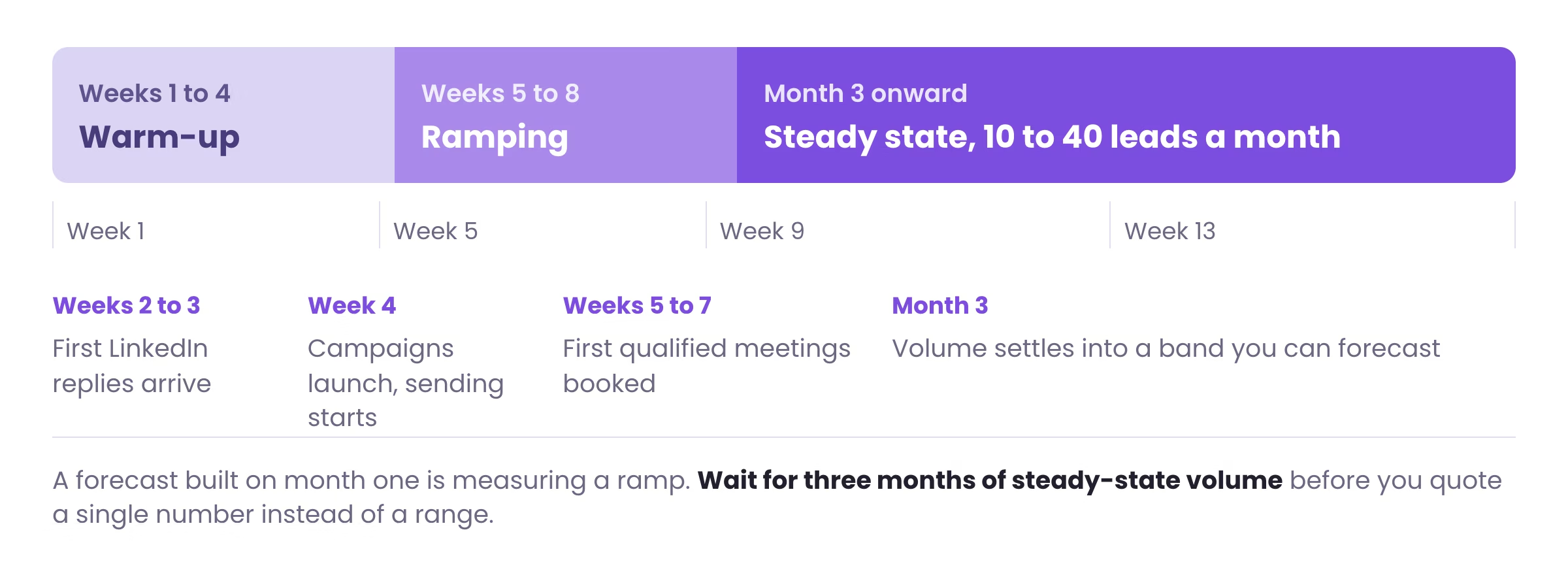
Three months. Infrastructure warm-up runs through week 4, LinkedIn replies start arriving in weeks 2 to 3, the first qualified meetings land between weeks 5 and 7, and volume settles into a predictable band from month 3. A forecast built on month one data will be wrong, because month one is a ramp and not a rate.
At steady state the range we work to is 5 to 50 highly interested leads per month depending on volume and market size. That band is the input for every model above. Once you have three months of it, the close rate and cycle length stop moving enough to matter and the forecast starts holding. Until then, forecast a range and label it a range.
If you would rather not spend a quarter building the measurement layer yourself, that is the work our outbound lead generation services cover, and our ROI calculator models the same ramp before you commit to anything.
Forecast a pipeline you can actually measure
We map your TAM, enrich it with live buying signals, and run the email, LinkedIn, and calling sequences that fill the top of the funnel. You get the conversion rates every model on this page needs, from a system we operate for you.
See how we book meetings
Sales forecasting examples: frequently asked questions
What is an example of sales forecasting?
A sales forecasting example is a projection built from measured conversion rates. On a published Reachly engagement, 85 qualified leads over six months converted to 6 closed deals, a 7.1% close rate. Carried forward at 14.2 leads per month, that forecasts 3 closed deals in the next quarter. Any forecast follows the same shape: a volume, a conversion rate, and a horizon.
What is the formula for calculating a sales forecast?
The simplest working formula is number of opportunities multiplied by average deal value multiplied by win rate. For pipeline velocity, divide that result by the sales cycle in days to get a daily run rate, then multiply by the days in your forecast period. With 40 opportunities, an $18,000 average deal, a 22% win rate, and a 75-day cycle, the daily figure is $2,112 and the quarter forecasts $190,080.
How do you do a sales forecast step by step?
Pull every open opportunity with its stage, value, and age. Calculate the historical close rate for each stage from at least two quarters of closed deals. Multiply each open deal by its stage close rate and add the results for a weighted number. Add new pipeline you expect to create in the period, using your own lead volume and meeting rate. Subtract deals already past your average cycle length, because they are stalled rather than pending. Publish the number as a range. Measure accuracy at the end of the period and adjust the rates.
What are the four types of forecasting?
The four most commonly used are qualitative forecasting from expert judgment, time series forecasting from historical patterns, causal or regression forecasting that ties revenue to driver variables, and simulation forecasting that runs multiple scenarios. B2B outbound teams usually combine time series for the base rate with causal modeling for buying signals.
What are the main sales forecasting models?
The nine models on this page cover the range most B2B teams need: pipeline velocity, intent-based demand forecasting, cohort analysis, territory and account-based forecasting, reply rate and engagement forecasting, regression and predictive modeling, multi-touch attribution, weighted pipeline by opportunity stage, and time series with moving averages. Weighted pipeline is the usual starting point because it reuses CRM stages you already have, and time series becomes useful once you hold at least three months of steady closed revenue.
What is the best forecasting method for sales?
For B2B outbound with a cycle under 90 days, pipeline velocity plus intent-based demand forecasting works best, because both read current pipeline behavior rather than last year's pattern. Teams with more than two years of clean CRM history and high deal volume get more from regression modeling. Teams with fewer than 50 deals a year should stay with weighted pipeline, since regression needs volume to be meaningful.
What are the 7 steps of forecasting?
Define the objective and the period. Choose the variables that move revenue. Gather and clean the historical data. Select the forecasting model that matches your data volume. Run the projection. Compare the output against actual results. Adjust the rates and repeat. The sixth step is the one most teams skip, and skipping it is why forecasts stay wrong for years.
How do you calculate forecast accuracy?
Subtract the forecast from actual revenue, take the absolute value, divide by actual revenue, then subtract that fraction from 1. A $250,000 forecast against $220,000 actual gives a $30,000 error, 13.6% of actual, so accuracy is 86.4%. Track it every period and chart the trend rather than judging a single quarter.
What is a good sales forecast accuracy rate?
Above 85% is a working forecast for most B2B teams. Between 70% and 85% the model is usable but the inputs need tightening, usually stage definitions or close-date hygiene. Below 70% the problem sits upstream in data quality or pipeline volume, and a different formula will not fix it.
What is an example of a marketing forecast?
A marketing forecast projects leads and pipeline from planned spend. Take $40,000 of quarterly budget at a measured $180 cost per lead: that returns 222 leads. If 12% historically become sales qualified, the forecast is 27 SQLs. Multiply by your close rate and average deal value to convert it into a revenue number the sales forecast can absorb.
What is an example of business forecasting?
Business forecasting covers any projection of future operating conditions. A financial example: $310,000 in the bank against a $46,000 monthly burn forecasts 6.7 months of runway. A workforce example: a $4M target at $800,000 quota per rep needs 5 quota-carrying reps, so 6 hires once you allow for ramp. Both use the same measure-then-project method as a sales forecast.
What are real life examples of forecasting?
Weather services projecting rainfall from atmospheric readings, retailers ordering inventory from last season's sell-through, airlines pricing seats from booking curves, and utilities sizing generation from temperature forecasts. Each takes an observed rate and extends it over a defined horizon, which is exactly what a sales forecast does with pipeline.
What is pipeline velocity and how do you calculate it?
Pipeline velocity is the rate at which revenue moves through your pipeline, expressed as dollars per day. Multiply open opportunities by average deal value and win rate, then divide by the average sales cycle in days. Its diagnostic value is higher than its forecasting value, because a drop tells you which of the four inputs moved and therefore which part of the process to fix.
How far ahead should a B2B sales forecast go?
One to two sales cycles. With a 75-day cycle that is roughly one to two quarters. Anything beyond two cycles depends on pipeline that does not exist yet, so it is a plan rather than a forecast. Forecast the current quarter from open pipeline and the next quarter from your lead generation rate, and keep the two numbers separate.
Why do most sales forecasts fail?
Three reasons account for most of it. Close dates get pushed rather than reset, so stalled deals stay in the current period. Stage close rates come from CRM defaults instead of measured history. And the top of the funnel is inconsistent, so there is no stable rate to project. The third is the most common, and it is a pipeline generation problem wearing a forecasting costume.
How long does outbound take before the pipeline is forecastable?
About three months. Campaigns launch from week 4 after infrastructure warm-up, LinkedIn replies arrive in weeks 2 to 3, first meetings come by week 5 to 6, or within 10 days on pre-warmed domains, and volume becomes predictable from month 3. Until then, forecast a range rather than a point, because early months are a ramp and not a steady rate.
Recommended service
B2B Appointment Setting Services
Reachly qualifies every reply for fit, authority, and intent, then books the meeting straight onto your calendar.